Programmatic usage (API)

The core class of nonos is GasDataSet that you need to import from nonos.api. GasDataSet takes the form:

ds = GasDataset(
    on,
    directory,
    geometry,
    code,
    inifile,
)

Mandatory argument:

on: output number (ex: for idefix, the VTK file f"data.{on:04d}.vtk")

Optional arguments:

directory: working directory where the output file is (default: current working directory).
geometry: if the geometry is not recognized.
code and inifile: if the parameter file is not recognized (i.e. different from idefix.ini for idefix, variables.par for fargo3d and pluto.ini for pluto). code can be "idefix", "fargo3d", "fargo-adsg" or "pluto".

GasDataSet is a field container, and you can access the fields in the form of a dictionary. You can check what fields are included in ds by running ds.keys(). For example, the density field could be accessed with ds["RHO"].

Examples

General case for the output number 0:
```
ds = GasDataset(0)
```
For a simulation with fargo-adsg and a parameter file "template.par" and for the output number 0, you need to do:
```
ds = GasDataset(
    0,
    code="fargo-adsg",
    inifile="template.par",
)
```
For a simulation performed with idefix in the directory "path/to/output", a parameter file "idefix-rkl.ini" and for the output number 10, you need to do:
```
ds = GasDataset(
    10,
    directory="path/to/output",
    code="idefix",
    inifile="idefix-rkl.ini",
)
```

Full examples

Example 1 (idefix, 2D, polar \(R\)-\(\phi\))

After going to the nonos directory, and opening ipython, we import GasDataSet.

import matplotlib.pyplot as plt
from nonos.api import GasDataSet

We use the class GasDataSet which takes as argument the output number of the output file given by idefix/pluto/fargo.

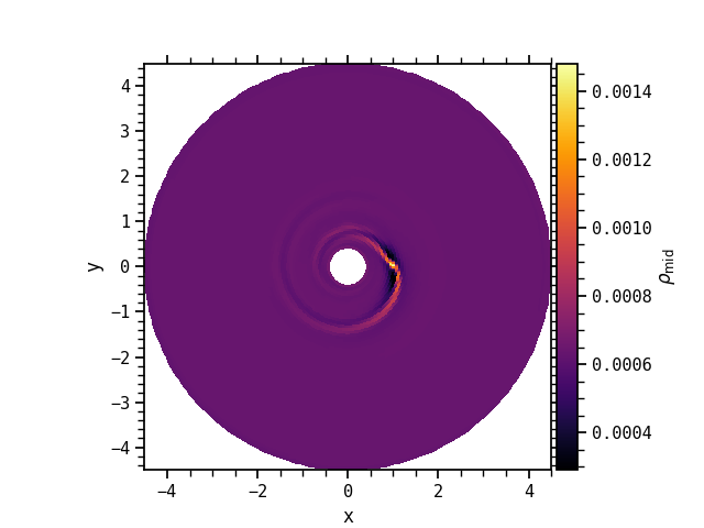
ds = GasDataSet(23, directory="tests/data/idefix_newvtk_planet2d")

As mentioned earlier, ds contains in particular a dictionary with the different fields. Let's say you want to perform a vertical slice of the density in the midplane, plot the result in the xy plane and rotate the grid given the planet number 0 (which orbit is described in the planet0.dat file):

dsvm = ds["RHO"].vertical_at_midplane().map("x", "y", rotate_with="planet0.dat")

dsop is now a Plotable object. We can e.g. represent its log10, with a given colormap, and display the colorbar by adding the argument title.

fig, ax = plt.subplots()
dsvm.plot(fig, ax, cmap="inferno", title=r"$\rho_{\rm mid}$")
ax.set_aspect("equal")
plt.show()

Example 2 (idefix, 3D, polar \(R\)-\(\phi\)-\(z\))

import matplotlib.pyplot as plt
from nonos.api import GasDataSet
ds = GasDataSet(43, geometry="polar", directory="tests/data/idefix_planet3d")

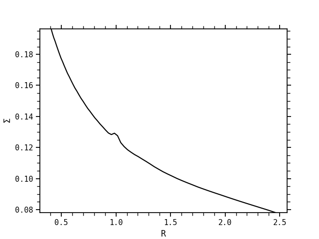
If now, with the same dataset, we perform a latitudinal projection of the field RHO, i.e. the integral of the density between \(-\theta\) and \(\theta\), and then an azimuthal average, before mapping it in the radial ("R") direction:

dslp = ds["RHO"].latitudinal_projection(theta=3*0.05).azimuthal_average().map("R")

Finally, we display the y-label by adding the argument title

fig, ax = plt.subplots()
dslp.plot(fig, ax, c="k", title=r"$\Sigma$")
plt.show()

rholpaa — Azimuthally-averaged surface density

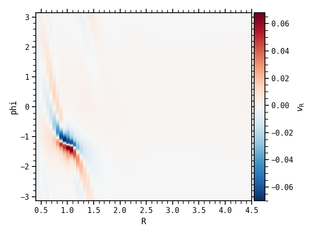
Example 3 (idefix, 2D, polar \(R\)-\(\phi\))

As a summary, we show here a simple 2D example.

import matplotlib.pyplot as plt
from nonos.api import GasDataSet
ds = GasDataSet(23, directory="tests/data/idefix_newvtk_planet2d")
fig, ax = plt.subplots()
ds["VX1"].map("R", "phi").plot(fig, ax, cmap="RdBu_r", title=r"$v_{\rm R}$")
fig.tight_layout()
plt.show()

Compute a new field

In order to compute a new field from preexisting ones, you can use the compute function, which takes 3 mandatory arguments (field the name of the new field, data the corresponding array and ref a known field with similar structure as the new field).

Example

Let us assume we have a VTK file named data.0000.vtk in cartesian geometry.

import numpy as np
from nonos.api import GasDataSet, compute

ds = GasDataSet(0)

Vnorm = compute(
  field="V",
  data=np.sqrt(ds["VX1"].data**2 + ds["VX2"].data**2 + ds["VX3"].data**2),
  ref=ds["VX1"],
)

Coordinates

If ds is a dataset, the coordinates ds.coords at the cell edges and cell centers can be accessed with the following attributes:

geometry	cartesian	polar	spherical
edges	(`x`, `y`, `z`)	(`R`, `phi`, `z`)	(`r`, `theta`, `phi`)
centers	(`xmed`, `ymed`, `zmed`)	(`Rmed`, `phimed`, `zmed`)	(`rmed`, `thetamed`, `phimed`)

Attributes of fields

If ds is a dataset containing the three-dimensional density field ds["RHO"], you can access important quantities, such as:

data: the 3D array.
coords: the coordinates that you can access depending on the geometry.
on: the output number associated with the VTK file.

Operations on fields

If ds is a dataset containing the three-dimensional density field ds["RHO"], several operations on the field are possible.

1. General operations

API function	operation	geometry
`latitudinal_projection(theta)`	Integral between \(-\theta\) and \(\theta\)	`polar`,`spherical`
`vertical_projection(z)`	Integral between \(-z\) and \(z\)	`cartesian`,`polar`
`vertical_at_midplane()`	Slice in the midplane	`cartesian`,`polar`,`spherical`
`latitudinal_at_theta(theta)`	Slice at latitude \(\theta\)	`polar`,`spherical`
`vertical_at_z(z)`	Slice at altitude \(z\)	`cartesian`,`polar`,`spherical`
`azimuthal_at_phi(phi)`	Slice at azimuth \(\phi\)	`polar`,`spherical`
`azimuthal_average()`	Azimuthal average	`polar`,`spherical`
`radial_at_r(distance)`	Slice at `distance`	`polar`,`spherical`
`radial_average_interval(vmin,vmax)`	Radial average (`vmin` to `vmax`)	`polar`,`spherical`

Chain the operations

Some of these operations can be combined, e.g. first a slice in the midplane and then an azimuthal average with ds["RHO"].vertical_at_midplane().azimuthal_average().

It is also possible to access some other quantities in the arrays:

API function	operation	geometry
`find_ir(distance)`	index in the radial direction at `distance`	`polar`,`spherical`
`find_imid(altitude)`	index in the \(z\)/\(\theta\) direction at `altitude`	`cartesian`,`polar`,`spherical`
`find_iphi(phi)`	index in the azimuthal direction at `phi`	`polar`,`spherical`

2. Other important operations

map("XDIR","YDIR"): before plotting the field, we have to map it in the ("XDIR","YDIR") plane + optional rotate_by (rotation angle, float) or rotate_with (planet log file, str) to rotate the grid. Mapping the field means here that we start with a native geometry for the outputs, e.g., a 2D polar geometry (\(R\), \(\phi\)), and we want to visualize it in a cartesian plane (\(x\), \(y\)). ("XDIR","YDIR") can be for example ("R","phi"), ("x","y"), ("x","z"), ("r","theta"),... depending on the native geometry you have and the target geometry you want.
diff(on): compute the relative difference of the same field for a different VTK file.
save(directory): create a .npy file which saves in directory the array you just computed.

3. Additional operations for planet / disk simulations

API function	operation	geometry
`azimuthal_at_planet(planet_number)`	Slice at planet azimuth \(\phi_p\)	`polar`,`spherical`
`remove_planet_hill(planet_number)`	Remove the Hill sphere	`polar`,`spherical`
`find_rp(planet_number)`	radial location of the planet	-
`find_rhill(planet_number)`	Hill radius of the planet	-
`find_phip(planet_number)`	azimuthal location of the planet	-

Remove the Hill sphere

remove_planet_hill(planet_number) masks the region \(\phi_p \in \left[\phi_p - 2 R_{\rm hill}/R_p , \phi_p + 2 R_{\rm hill}/R_p \right]\) with \((R_p, \phi_p)\) the planet's coordinates and \(R_{\rm hill}\) its Hill radius.

4. Save fields and read dataset from reduced files

It is possible to save reduced arrays in NPY files, which are standard binary file format for numpy arrays. It it then possible to get a dataset from these reduced files. It could be a good strategy to pre-process large VTK files on a cluster and transfer afterwards the reduced files locally for post-processing.

Save reduced fields (idefix, 3D, spherical \(r\)-\(\theta\)-\(\phi\))

from nonos.api import GasDataSet
ds = GasDataSet(500, directory="tests/data/idefix_spherical_planet3d")
for field in ("RHO", "VX1"):
    ds[field].azimuthal_average().save("tests/data/idefix_spherical_planet3d")

Access reduced fields in a dataset (idefix, 3D, spherical \(r\)-\(\theta\)-\(\phi\))

from nonos.api import GasDataSet
ds_aa = GasDataSet.from_npy(500, operation="azimuthal_average", directory="tests/data/idefix_spherical_planet3d")

Plotting the fields

Once the field has been mapped in a plane of visualization (ex: dsmap = ds["RHO"].radial_at_r(1).map("phi","z")), we can plot it using the plot method. Note that you first need to create your figure and subplots, and you can afterwards add some complexity by using the power of matplotlib.

Mandatory arguments:

fig and ax: matplotlib figure and subplot (ex: fig, ax = plt.subplots())

Optional arguments:

log: plot the log10 of the field (default: False)
vmin and vmax: set respectively the minimum value and maximum value of the data
cmap: choice of colormap (default: inferno)
title: name of the field in the colorbar (default: None, i.e. no colorbar)
filename, fmt and dpi: in order to directly save the plot, corresponds respectively the name of the file, the extension (default: png) and the resolution (default: 500) of the saved figure. It is equivalent to
```
plt.savefig(f"{filename}.{fmt}", bbox_inches="tight", dpi=dpi)
```
By default, the figure is not saved in case you want to personalize the final plot with other matplotlib operations.

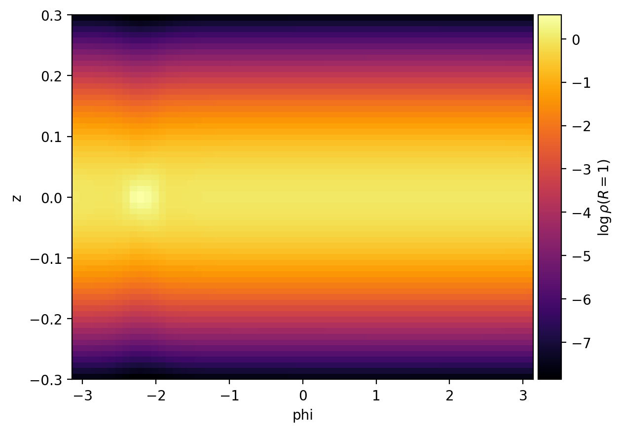
Plotting a file (idefix, 3D, polar \(R\)-\(\phi\)-\(z\))

import matplotlib.pyplot as plt
from nonos.api import GasDataSet

ds = GasDataSet(23)
dsmap = ds["RHO"].radial_at_r(1).map("phi","z")
fig, ax = plt.subplots()
dsmap.plot(
    fig,
    ax,
    log=True,
    title=r"$\rho(R=1)$",
    filename="rho_R1",
    fmt="png",
    dpi=200,
)

rhor_phiz — Density in the plane \(\phi\)-\(z\)